球状の空隙をもつ材料の、空隙モデルをボクセル形式で生成しました。
まずはライブラリをインポート。
import numpy as np
from numpy.random import randint
import pandas as pd
import matplotlib.pyplot as plt
from mpl_toolkits.mplot3d import Axes3D
from skimage.morphology import ball
import random
import tqdm

np.set_printoptions(edgeitems=5)
球状空隙は、skimage.morphology.ball()で生成します。
fig = plt.figure(figsize=(8, 8))

ax = fig.add_subplot(1, 1, 1, projection=Axes3D.name)
ax.voxels(ball(5))

fig.tight_layout()
plt.show()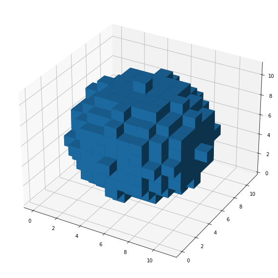
空隙を発生させる範囲は、1辺500pxの立方体を用意します。
sample = np.zeros((500,500,500))
print(sample.shape)
# (500, 500, 500)
立方体と空隙半径を引数に、立方体内のランダムな位置かつ、空隙同士が重ならないように空隙を生成する関数を定義します。
def generate_ball(sample, radius):
    x_max, y_max, z_max = sample.shape
    xs, ys, zs = np.where(sample[radius:x_max-radius, radius:y_max-radius, radius:z_max-radius]==0)

    for i in range(1000):
        rand_num = randint(len(xs))
        x, y, z = xs[rand_num]+radius, ys[rand_num]+radius, zs[rand_num]+radius

        # 重なりチェック
        exist = sample[x-radius:x+radius+1,y-radius:y+radius+1,z-radius:z+radius+1][ball(radius).astype('bool')].sum()
        if exist==0:
            sample[x-radius:x+radius+1,y-radius:y+radius+1,z-radius:z+radius+1] += ball(radius)
            # print('(x,y,z)= ',x,y,z,', radius= ',radius)
            return sample, x, y, z

    ind_li = list(range(len(xs)))
    random.shuffle(ind_li)
    for i in ind_li[:1000]:
        x, y, z = xs[i]+radius, ys[i]+radius, zs[i]+radius

        # 重なりチェック
        exist = sample[x-radius:x+radius+1,y-radius:y+radius+1,z-radius:z+radius+1][ball(radius).astype('bool')].sum()
        if exist==0:
            sample[x-radius:x+radius+1,y-radius:y+radius+1,z-radius:z+radius+1] += ball(radius)
            # print('(x,y,z)= ',x,y,z,', radius= ',radius)
            return sample, x, y, z
半径30pxの均一な球状空隙を空隙率が25%以上となるまで繰り返し生成させます。
# 半径30の球を繰り返し生成
np.random.seed(0)
random.seed(0)

sample = np.zeros((500,500,500))
w,h,c=sample.shape
print('ball_volume: ', ball(30).sum())
print('before_volume: ', sample.sum())
re_li = []

for i in tqdm.tqdm(range(400)):
    sample,x,y,z = generate_ball(sample, 30)
    re_li.append([30,x,y,z])
    if (sample.sum()/(w*h*c)*100)>25:
        break

print('after_volume: ',sample.sum())
print('filled(%): ', sample.sum()/(w*h*c)*100)

pd.DataFrame(re_li, columns=['radius','x','y','z']).to_csv('gen_ball_uniform.csv')
np.save('gen_ball_uniform', sample)

plt.imshow(sample[:,:,100])
plt.show()
plt.imshow(sample[:,:,200])
plt.show()
ball_volume: 113081
before_volume: 0.0
69%|██████▉ | 276/400 [03:32<01:35, 1.30it/s]
after_volume: 31323437.0
filled(%): 25.058749600000002

スライス画像から、ちゃんと生成されていることが分かります。
続いて、球状空隙の体積が正規分布に従うように、25%以上となるまで繰り返し生成させます。ここで、正規分布の平均・標準偏差を半径30pxの球体の体積(px^3)とします。
# 半径が正規分布(v_30, v_30)に従う球を繰り返し生成
np.random.seed(0)
random.seed(0)
rate = 1
volume_30 = np.pi*4*(30**3)/3

sample = np.zeros((500,500,500))
w,h,c=sample.shape
print('before_volume: ', sample.sum())
re_li = []

for i in tqdm.tqdm(range(500)):
    volume = np.random.randn()*volume_30*rate + volume_30
    if volume<0:
        continue
    radius = round((volume*3/4/np.pi)**(1/3))
    sample,x,y,z = generate_ball(sample, radius)
    re_li.append([radius,x,y,z])
    if (sample.sum()/(w*h*c)*100)>25:
        break

print('after_volume: ',sample.sum())
print('filled(%): ', sample.sum()/(w*h*c)*100)

pd.DataFrame(re_li, columns=['radius','x','y','z']).to_csv(f'gen_ball_gauss_mu30v_sigma{rate:.1f}v.csv')
np.save(f'gen_ball_gauss_mu30v_sigma{rate:.1f}v', sample)

plt.imshow(sample[:,:,100])
plt.show()
plt.imshow(sample[:,:,200])
plt.show()
before_volume: 0.0
50%|████▉ | 248/500 [07:52<08:00, 1.91s/it]
after_volume: 31278078.0
filled(%): 25.022462400000002

均一な空隙よりも、スライス画像の断面円の大きさがまばらになっています。
続いて、生成された空隙の半径と、スライス画像から見た断面円の半径のヒストグラムを確認します。
slice_li = [100, 150, 200, 250, 300, 350, 400]

for file in file_li:
    print(file)
    df = pd.read_csv(file, index_col=0)
    df['volume'] = 4*np.pi/3*(df['radius']**3)
    re_li = []

    for slice_z in slice_li:
        df[f'slice_{slice_z}'] = (df['z'] - slice_z).abs()< df['radius']
        df[f'slice_{slice_z}_r'] = 0

        tmp = df[df[f'slice_{slice_z}']]
        df.loc[df[f'slice_{slice_z}'],f'slice_{slice_z}_r'] = (tmp['radius']**2 - (tmp['z'] - slice_z)**2)**(1/2)
        re_li.append(df[df[f'slice_{slice_z}']][f'slice_{slice_z}_r'])

    df.to_csv(file)

    print('true std: ',df['radius'].std())
    print('slice std: ', pd.concat(re_li).std())

    r_min = min(df['radius'].min(), pd.concat(re_li).min())
    r_max = max(df['radius'].max(), pd.concat(re_li).max())
    delta = r_max - r_min

    fig = plt.figure(figsize=(6, 9))

    fig.align_ylabels()

    ax = fig.add_subplot(3, 1, 1)
    ax.hist(df['volume'], label='true', color='royalblue', bins=10)
    ax.set_ylabel('frequency')
    ax.set_xlabel('volume (px^3)')
    plt.legend()

    ax = fig.add_subplot(3, 1, 2)
    ax.hist(df['radius'], label='true', color='royalblue', range=(r_min, r_max), bins=10)
    ax.set_xlim(r_min - delta*0.05, r_max + delta*0.05)
    ax.set_ylabel('frequency')
    ax.set_xlabel('radius (px)')
    plt.legend()

    ax = fig.add_subplot(3, 1, 3)
    ax.hist(pd.concat(re_li), label='slice', color='darkorange', range=(r_min, r_max), bins=10)
    ax.set_xlim(r_min - delta*0.05, r_max + delta*0.05)
    ax.set_ylabel('frequency')
    ax.set_xlabel('radius (px)')
    plt.legend()

    fig.tight_layout()
    plt.show()
均一空隙を生成
true std:  0.0
slice std:  6.675737173960232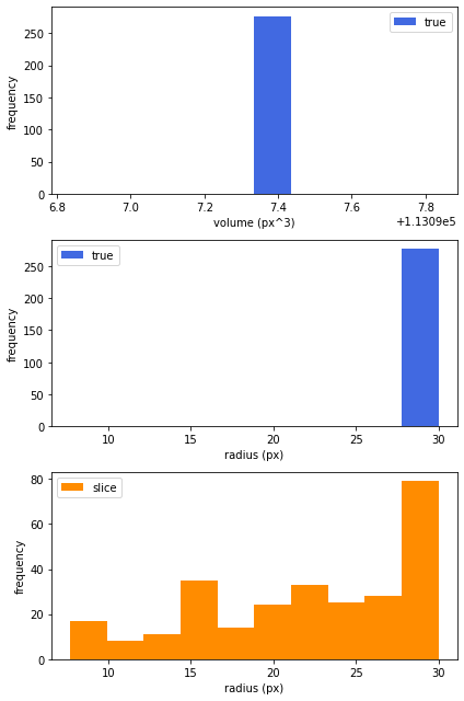
正規分布から生成
true std:  7.980581633143674
slice std:  9.261831317960853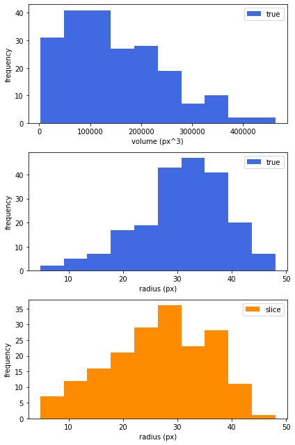
どちらも、断面円の半径は実際の空隙半径に対して小さく観測されることが確認できました。


コメント