LiNGAMを使って因果探索

diabetesデータセットを使ってLiNGAMで因果探索をやってみたメモです。

LiNGAMチュートリアル

DirectLiNGAM — LiNGAM 1.8.0 documentation

lingam.readthedocs.io

diabetesデータセット

sklearn.datasets.load_diabetes

Examples using sklearn.datasets.load_diabetes: Release Highlights for scikit-learn 1.2 Gradient Boosting regression Plot individual and voting regression predic...

scikit-learn

内容

準備

# ライブラリインポート
import pandas as pd
import numpy as np

from sklearn.datasets import load_diabetes
from sklearn.preprocessing import StandardScaler

import graphviz
import lingam
from lingam.utils import make_dot, make_prior_knowledge

# データセット読み込み
dataset = load_diabetes(as_frame=True)['data'][['age', 'sex', 'bmi', 'bp']]
dataset['target'] = load_diabetes(as_frame=True)['target']
dataset.head()

　　　　　　　age	　　　sex	　　　bmi	　　　bp	target
0	0.038076	0.050680	0.061696	0.021872	151.0
1	-0.001882	-0.044642	-0.051474	-0.026328	75.0
2	0.085299	0.050680	0.044451	-0.005671	141.0
3	-0.089063	-0.044642	-0.011595	-0.036656	206.0
4	0.005383	-0.044642	-0.036385	0.021872	135.0

DirectLiNGAMで因果探索

# 標準化
scaler = StandardScaler()
Xy = scaler.fit_transform(dataset)

# モデル作成
model = lingam.DirectLiNGAM(random_state=1)
model.fit(Xy)

# 因果の順番
print(model.causal_order_)

# 隣接行列
print(model.adjacency_matrix_)

# 推定した因果モデルにおける、誤差同士の独立性のp値
p_values = model.get_error_independence_p_values(Xy)
print(p_values)

[1, 4, 0, 3, 2]

[[0.         0.16595397 0.         0.         0.18074244]
 [0.         0.         0.         0.         0.        ]
 [0.         0.         0.         0.13460604 0.47664595]
 [0.23008202 0.1842314  0.         0.         0.39032065]
 [0.         0.         0.         0.         0.        ]]

[[0.         0.59336161 0.01471721 0.77585358 0.26328001]
 [0.59336161 0.         0.00190972 0.44643012 0.73256818]
 [0.01471721 0.00190972 0.         0.03910181 0.00928811]
 [0.77585358 0.44643012 0.03910181 0.         0.31827615]
 [0.26328001 0.73256818 0.00928811 0.31827615 0.        ]]

# 因果グラフの描画
# 以下よりgraphvizのexeをインストールする。インストール時にpathに追加する。
# https://graphviz.org/download/

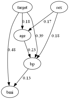
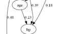
dot = make_dot(model.adjacency_matrix_, labels=dataset.columns.to_list())
dot.format = 'png'
dot.render('DirectLiNGAM')
dot

ICA-LiNGAMで因果探索

# 標準化
scaler = StandardScaler()
Xy = scaler.fit_transform(dataset)

# モデル作成
model = lingam.ICALiNGAM(random_state=1)
model.fit(Xy)

# 因果の順番
print(model.causal_order_)

# 隣接行列
print(model.adjacency_matrix_)

# 推定した因果モデルにおける、誤差同士の独立性のp値
p_values = model.get_error_independence_p_values(Xy)
print(p_values)

[0, 1, 2, 4, 3]

[[0.         0.         0.         0.         0.        ]
 [0.1737371  0.         0.         0.         0.        ]
 [0.11730318 0.         0.         0.         0.        ]
 [0.2186471  0.17565042 0.16626303 0.         0.29533368]
 [0.06725074 0.         0.55633393 0.         0.        ]]

[[0.00000000e+00 5.22387240e-28 6.13151850e-03 4.23593615e-01
 5.80968024e-02]
 [5.22387240e-28 0.00000000e+00 3.45693925e-05 4.28599682e-01
 3.50082931e-01]
 [6.13151850e-03 3.45693925e-05 0.00000000e+00 2.83284247e-01
 1.52685320e-09]
 [4.23593615e-01 4.28599682e-01 2.83284247e-01 0.00000000e+00
 7.24168274e-01]
 [5.80968024e-02 3.50082931e-01 1.52685320e-09 7.24168274e-01
 0.00000000e+00]]

dot = make_dot(model.adjacency_matrix_, labels=dataset.columns.to_list())
dot.format = 'png'
dot.render('ICALiNGAM')
dot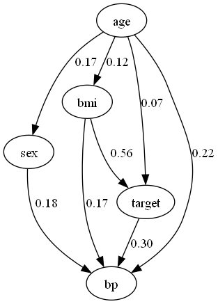

LiNGAMのアルゴリズムによって、推論結果がかなり異なってますね。また、ageとsexに有向辺があることから、データセット自体のバイアスもうかがえます。

時前知識の導入

DirectLiNGAMでは事前知識を導入することができます。

How to use prior knowledge in DirectLiNGAM — LiNGAM 1.8.0 documentation

lingam.readthedocs.io

# 事前知識のグラフを描画する関数
def make_prior_knowledge_graph(prior_knowledge_matrix):
    d = graphviz.Digraph(engine='dot')

    labels = [f'x{i}' for i in range(prior_knowledge_matrix.shape[0])]
    for label in labels:
        d.node(label, label)

    dirs = np.where(prior_knowledge_matrix > 0)
    for to, from_ in zip(dirs[0], dirs[1]):
        d.edge(labels[from_], labels[to])

    dirs = np.where(prior_knowledge_matrix < 0)
    for to, from_ in zip(dirs[0], dirs[1]):
        if to != from_:
            d.edge(labels[from_], labels[to], style='dashed')
    return d

# 事前知識の隣接行列を作成
prior_knowledge = make_prior_knowledge(
    n_variables=5,
    sink_variables=[4],
)
print(prior_knowledge)

# 事前知識のグラフを描画
dot = make_prior_knowledge_graph(prior_knowledge)
dot.format = 'png'
dot.render('prior_knowledge')
dot

[[-1 -1 -1 -1  0]
 [-1 -1 -1 -1  0]
 [-1 -1 -1 -1  0]
 [-1 -1 -1 -1  0]
 [-1 -1 -1 -1 -1]]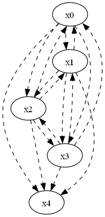

# 標準化
scaler = StandardScaler()
Xy = scaler.fit_transform(dataset)

# モデル作成
model = lingam.DirectLiNGAM(random_state=1, prior_knowledge=prior_knowledge)
model.fit(Xy)

# 因果の順番
print(model.causal_order_)

# 隣接行列
print(model.adjacency_matrix_)

# 推定した因果モデルにおける、誤差同士の独立性のp値
p_values = model.get_error_independence_p_values(Xy)
print(p_values)

[1, 0, 2, 3, 4]

[[0.         0.1737371  0.         0.         0.        ]
 [0.         0.         0.         0.         0.        ]
 [0.11730318 0.         0.         0.         0.        ]
 [0.24398632 0.16905852 0.33535276 0.         0.        ]
 [0.         0.         0.45350717 0.21372887 0.        ]]

[[0.00000000e+00 3.60143516e-01 4.92456030e-02 2.44043685e-03
 1.81716999e-01]
 [3.60143516e-01 0.00000000e+00 2.28878413e-04 4.73044868e-01
 1.92837115e-01]
 [4.92456030e-02 2.28878413e-04 0.00000000e+00 4.94064284e-02
 3.81145593e-07]
 [2.44043685e-03 4.73044868e-01 4.94064284e-02 0.00000000e+00
 1.48929893e-01]
 [1.81716999e-01 1.92837115e-01 3.81145593e-07 1.48929893e-01
 0.00000000e+00]]

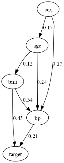
dot = make_dot(model.adjacency_matrix_, labels=dataset.columns.to_list())
dot.format = 'png'
dot.render('DirectLiNGAM_w/prior_knowledge')
dot

事前知識あり

事前知識無し

事前知識を導入することで、targetが因果関係の中継地点、又は終点であるという仮定の下で因果探索することができました。

Bootstrap

ブートストラップ法の概要：

1. 元データからn個の標本を復元抽出する。このときnは元データの標本数である。
2. 統計モデル（モデルパラメータ）を推定する。
3. このブートストラップ抽出を何度も（B回）繰り返す。
4. こうして計算された「推定量の標本分布」は、本来の標本分布の近似になっている。

Bootstrap — LiNGAM 1.8.0 documentation

lingam.readthedocs.io

from lingam.utils import print_causal_directions, print_dagc

scaler = StandardScaler()
Xy = scaler.fit_transform(dataset)

model = lingam.DirectLiNGAM(random_state=1, prior_knowledge=prior_knowledge)
result = model.bootstrap(Xy, n_sampling=100)
# sklearn.utils.resampleで重複ありのリサンプリングをしている。リサンプル後のサンプル数は元データと同じ。

# bootstrappingの各サンプルにおける、因果方向の有無のカウント結果を取得する
cdc = result.get_causal_direction_counts(n_directions=8, min_causal_effect=0.01, split_by_causal_effect_sign=True)
print_causal_directions(cdc, 100, labels=dataset.columns.to_list())

# カウント結果を確率として、隣接行列の形式で表示
prob = result.get_probabilities(min_causal_effect=0.01)
print(prob)

p <--- sex (b>0) (100.0%)
target <--- bmi (b>0) (100.0%)
target <--- bp (b>0) (100.0%)
bp <--- age (b>0) (93.0%)
age <--- sex (b>0) (83.0%)
bp <--- bmi (b>0) (82.0%)
bmi <--- age (b>0) (79.0%)
target <--- sex (b<0) (47.0%)

[[0.   0.83 0.02 0.07 0.  ]
 [0.   0.   0.   0.   0.  ]
 [0.79 0.3  0.   0.18 0.  ]
 [0.93 1.   0.82 0.   0.  ]
 [0.18 0.47 1.   1.   0.  ]]

# bootstrappingの各サンプルにおける、DAG(Directed Acyclic Graphs)のカウント結果を取得する
dagc = result.get_directed_acyclic_graph_counts(n_dags=3, min_causal_effect=0.01, split_by_causal_effect_sign=True)
print_dagc(dagc, 100, labels=dataset.columns.to_list())

DAG[0]: 18.0%
	age <--- sex (b>0)
	bmi <--- age (b>0)
	bp <--- age (b>0)
	bp <--- sex (b>0)
	bp <--- bmi (b>0)
	target <--- bmi (b>0)
	target <--- bp (b>0)
DAG[1]: 14.0%
	age <--- sex (b>0)
	bmi <--- age (b>0)
	bp <--- age (b>0)
	bp <--- sex (b>0)
	bp <--- bmi (b>0)
	target <--- sex (b<0)
	target <--- bmi (b>0)
	target <--- bp (b>0)
DAG[2]: 9.0%
	age <--- sex (b>0)
	bmi <--- age (b>0)
	bmi <--- sex (b>0)
	bp <--- age (b>0)
	bp <--- sex (b>0)
	bp <--- bmi (b>0)
	target <--- sex (b<0)
	target <--- bmi (b>0)
	target <--- bp (b>0)

# Total Causal Effects
causal_effects = result.get_total_causal_effects(min_causal_effect=0.01)

# Assign to pandas.DataFrame for pretty display
df = pd.DataFrame(causal_effects)
labels = dataset.columns.to_list()
df['from'] = df['from'].apply(lambda x : labels[x])
df['to'] = df['to'].apply(lambda x : labels[x])
df

	from	to	effect	probability
0	sex	bp	0.222785	1.00
1	bmi	target	0.553888	1.00
2	bp	target	0.246653	1.00
3	age	bp	0.309844	0.93
4	age	target	0.166742	0.88
5	age	bmi	0.162367	0.84
6	sex	age	0.187258	0.83
7	bmi	bp	0.351166	0.82
8	sex	bmi	0.135094	0.27
9	bp	bmi	0.325201	0.18
10	bp	age	0.369898	0.07
11	sex	target	0.136603	0.04
12	bmi	age	0.194196	0.02